A

Macro Approach To

Detection and Prevention of Corporate Insolvency

(The Determinant Factors)

Enyi Patrick Enyi (ACCA, ACA, MBA)

Head, Department of Accounting

Madonna University, Okija - Onitsha

Anambra State, Nigeria.

TITLE PAGE

TITLE of PAPER: A “MACRO” APPROACH TO DETECTION AND PREVENTION OF CORPORATE INSOLVENCY

(The Determinant factors.)

ABSTRACT

The application of financial analysis tools such as current, quick, and fixed assets ratios, creditors cover and liquidity index among others have not helped in stemming the rising rate of insolvency and business liquidation owing mainly to the fact that these tools are inadequately equipped to highlight futuristic financial problem spots. A normative research carried out on moribund business organizations in Nigeria aimed at finding the reasons for their inability to detect futuristic financial problem spots and proffering solutions thereon reveal that there are factors other than immediate liquidity considerations which also affect the “going concern” position of a business in the long run. It also revealed that every business has its operational point of perfection, which stands as its financial homeostasis and that three main variables (product mark-up ratio, technical efficiency level, and the cost of operating a production cycle) are necessary for proper estimation of working capital adequacy. The study made use of the experimental and survey research methods for internal and external validity tests respectively. It recommends the application of an advanced working capital “formula” derived from this study for estimating the most appropriate level for a firm’s working capital base, as well as predict organizational life-span and evaluate future projects more objectively.

INTRODUCTION

The last 20 years witnessed a spate of entrepreneurial turbulence unprecedented in the more than 40 years history of business entrepreneurship in independent Nigeria. The rate at which business sprang up and go under was and is still of much concern to the average discerning entrepreneur. Worst hit in this wave of financial misfortune are banks and their hapless depositors/customers. According to Business Times vol.6 No 12, 2002, as much as 5 banks are currently listed as distressed and could be liquidated any moment. The cause of course is Insolvency.

The first stage in liquidation starts with insolvency. For clarity we define insolvency as the inability of an organization to meet the demands of its maturing current or long term liabilities owing to lack of liquid funds. It is obvious from the job descriptions of business managers that they are responsible for the detection and prevention of insolvency in their firms. The ability to do this lies squarely on how the firm’s working capital resources is managed (Enyi 2002).

Sellers et al (2002) in analysing the decisions of Canadian courts on insolvency tried to distinguish between corporate insolvency, liquidity and balance sheet insolvency defined insolvency thus:

Insolvency occurs when

- a corporation is unable to meet its obligation as they generally come due;

- a corporation has ceased meeting obligations as they generally come due;

- the property of the corporation at a fair value is not sufficient to enable payment of all obligations due and accruing due.

Thus, the first type of insolvency, they referred to as “corporate insolvency”, the second, they tagged “Liquidity insolvency” and the last they called “Balance sheet insolvency”.

Doetsch and Hammer (2002) identified another type of insolvency which they called “Cross Border Insolvency”. Cross Border Insolvency according to them exist where transnational firms are unable to generate sufficient revenue to satisfy their debt obligations. Their financial distress then creates a situation where assets and claimants are scattered across more than one country.

To manage working capital along line entrepreneurial objectives, finance and business activity controllers employ the use of tools such as ratio analysis, forecasting and budgetary controls, among others. These tools combine to give the business managers historical as well as predictive information, which they need for their day-to-day job of making survival decisions for their organization. The ability to get the right information at the right time and to take the right decision where and when if matters most confers a big advantage on the firm over its peers and go a long way to determine the eventual survival and success of such an organisation.

The main problem facing business managers and that which this paper aims to tackle is of course, the usual lack of the right information at the right time and most likely too, the absence or non-existing predictive information generation tool such as the one that could reveal futuristic financial problem spots. To buttress this latter assertion, a look at the current financial analysis tools will point out the obvious defects in them.

Present Attempts At Predicting Insolvency

Information relating to business survival and insolvency are normally derived using the following ratio analysis:

1. Working Capital Ratio: This is a loose measure of capital adequacy or insolvency, which considers the totality of current assets as against the totality of current liabilities existing at a particular point (VanHorne 1977)

2. Quick (Acid Test) Ratio: This is a tighter measure of capital adequacy or insolvency, which considers only cash and near cash assets against the totality of current liabilities. This is what is currently and erroneously referred to as the “Solvency Ratio”. (This assertion shall be proved as we progress).

3. Fixed Assets Ratio: This ratio is another loose measure of capital adequacy, which is intended to weigh the available working capital against the totality of fixed assets apparently hoping to measure the proportion of the firm’s working capital that is available for servicing the fixed capital of the organization (Osisioma 1997).

Other measures of capital adequacy include; Creditors Cover and Liquidity Index, which have little significance in detecting especially, long term solvency of an organization. There are other measures associated with working capital, which ostensibly are also intended to equip managers with facts and data concerning the financial livewire of their organisation.

In all, these existing tools are at best a kid’s glove approach to working capital management. This is because most of them mainly lay emphasis on short-term solvency as expressed in the relationship between available current assets and their ability to offset current liabilities as they fall due. The present approach systematically ignores the future requirements of the firm. This situation is what can aptly be termed as the “micro” approach to working capital management, and this particularly seemed not to realize even as glaring as it is, that there is something, a powerful factor which determines the extent of success and longevity of a business organization from the onset and which continued to play a role throughout the life of the organization, metamorphosing from one problem type into another in the all apparent response to the dictum of economic and social manipulations. This obviously calls for a “macro” approach, which will look at the entire working capital need of a firm in terms of the foreseeable size of the firm’s activities given the organization’s initial level of technical and managerial efficiency. This is the missing link that this article intends to provide.

The first attempt to, perhaps, suggest a more effective way of preventive business failure forecasting was in the works of Altman (1983) in which he used the discriminate analysis technique to calculate bankruptcy ratio. This ratio which uses the Z value to represent over all index of corporate fiscal health, is used mostly by stockholders to determine if the company is a good investment. The formula for the ratio is

Z = 1.2X₁ + 1.4X₂ + 3.3 X₃+ 0.6X₄ + 1.0X₅

where

X₁ = Working capital divided by total assets

X₂ = Retained earnings divided by total assets

X₃ = Earnings before interest and taxes divided by total assets

X₄ = Market value of equity divided by the book value of total of total debt.

X₅ = Sales divided by total assets.

The range of the Z-value for most corporations is between -4 and +8.

According to Altman (1983), financially strong corporations have Z values above

2.99 while those in serious trouble have Z- value below 1.81. Those in the

Middle are question marks that could go either way. The closer the firm gets to bankruptcy/insolvency, the more accurate the Z value is as a predictor.

A critical look at the components of the Altman’s Z value formula and the interpretations reveal that, though the Z-value ratio is a milestone in the prediction of corporate insolvency, it suffers in precision and is likely to mislead the user unless, and off course, the corporation under analysis has already reached the problem spot. Also, more confusing is the range of acceptable values, users would perhaps, have preferred Z-value set in fractions or percentages as these are more or less universal and better understood than the ones used. Though, Altman rightly included working capital, retained earnings and earning before interest and taxes in his analysis as these are the main, if not the only, determinants of corporate solvency, the inclusion of such items as market value of share and total sales serves little or no purpose in the determination of the corporate solvency. This is because you can make billions of Naira of sales and yet record losses; and as posited earlier, it is profits that fuel continued cash flow, losses only dwindle them. In the same vein, the market value of a company’s share is external and has nothing to contribute to either profitability or cash flow. Hence, the inclusion of these two in the analysis only goes further to confuse the consequent Z-value outcome.

Business solvency revolves primarily at the working capital base of the organization, the fixed assets are only called upon at the critical but more agonizing stage of dismemberment when the death throws have already set in. The objective of any predictive function is to fore warn about a situation so that it can be avoided or taken advantage of. When this is lacking in a tool, then the tool becomes ineffective. Nevertheless, Altman’s work is still a very useful reference point in the analysis and study of business insolvency.

Capitalization

The foundation of all business enterprises lies on the capital base of the organisation. In fact, the business organization is as large as its capital base and as strong as its earning capacity (Enyi 2002). Capital can be defined as the amount set-aside for the establishment and running of a business organisation. To the economist, capital is a resource set aside for the production of future goods and other resources, (Samuelson 1980:45).

Osisioma (1997) identifies the two types of capital as fixed and circulating capital (the latter we commonly refer to as working capital). Whichever types of capital a business has, matters much less to the survival of the business than the adequacy of such capital and how they are managed. He stated that while the investor will be primarily interested in the fixed capital of an enterprise, the creditors will attach more importance on the nature and adequacy of the firm’s working capital as this is the area that bothers on whether and how they get paid.

The American Accounting Research Bulletin No. 43 in Osisioma (1997) defined Working capital as a “margin or buffer for meeting obligations within the ordinary operating cycle of the business”.

Working Capital Management.

VanHorne (1977) described working capital management as the administration of current assets in the name of cash, marketable securities, receivables and inventories whilst Osisioma B.C. (1997) defined it as the regulations, adjustment and control of the balances of current assets and current liabilities of a firm such that maturing obligations are met, and the fixed assets are properly serviced.

Working Capital Adequacy

To be adequate, working capital must be supplied in Desirable Quantities while maintaining Necessary Components. The size of a firm’s working capital is determined by a number of critical factors. The first being the size and scope of the business operations. The adequacy of any working capital is closely tied to the size and scope of the organization’s operations. Other factors that determine adequacy include the length of the production cycle. For the purpose of this article, we shall promptly refer to the “Production cycle” mentioned within the preceding paragraphs henceforth or interchangeably as “production run” or production trial”. Hence, a production run is hereby defined as

The lowest recognizable periodic division of an organisation’s production and marketing activities which can be quantified on the basis of cost and income, upon which budgets and projections can be prepared.

For elaboration, if a firm produces 100 articles per day from a cycle of 20 production activities, this will give 5 articles per production. It may just suffice to say that one production run makes up to 5 articles, however; this may not be ideal as there are some costs that follow defined periods. E.g. wages; and apportioning them to each production cycle may be a bit misleading. The most ideal thing to do would be to aggregate all productions and cost for one day and treat them as “one production run”.

The liquidity approach is the most effective way of measuring working capital adequacy in the short run; this of course, is the universal approach. However, with liquidity defined as “ability to realize value in money....”, (Van Horne 1977); we should concern ourselves with the continued promotion of the “going concern” principle for the organization by choosing a MACRO approach towards the firm’s working capital requirements rather than the micro method. This is the net-investment approach.

A measure of working capital adequacy which uses the net-investment approach and particularly avoiding all static components should strive at a position which adequately pinpoints the actual working capital requirement of the firm at any future point in time, given present and any future projected changes in the firm’s activity level, as well as the inflationary trend of the economy. This is because management and investors are more concerned with future periods than with the present and past. A more suitable measure should include a system that will take into consideration the past and present (as a guide) and the future (as a plan) to arrive at its result. This is the area where the existing solvency measurement tools have grossly been found wanting.

Learning Curves

C.T. Horngren (1982) in his words defined Learning Curve as “a cost function where average costs per unit of output decline systematically as cumulative production rises”. The connection between learning curve and working capital management stems from the fact that faulty productions owing to inexperience adds to costs in the same way as the longer time it takes a new comer to a task which results in higher wage payments than when such tasks were undertaken by a highly experienced worker.

More so, a study on the capital adequacy of small firms indicated that loses arising from the cost of learning do, in fact, contribute to capital depletion. The longer the period of learning, the higher the cost associated with learning and the more the organisation’s capital is depleted. How badly this will affect the organization will depend, to a large extent, on the rate of cost/loss recovery as expressed in the pricing/marketing ability of the organisations goods and services.

Of course, it will take an organization with a lower price-to-cost mark-up ratio much longer period to fully recover costs and losses associated with the learning period than it would take a similar organisation with the same learning period but with much higher mark-up ratio. Thus, the costs and losses associated with the learning periods can adversely affect the solvency of an organisation when:

Ø The learning period is unusually long and/or the mark-up ratio is too low to hasten recovery of cost and learning losses;

Ø The learning period is short but no adequate capital to continue production and enhance the recovery of costs and learning losses or a combination.

METHODOLOGY

Two research methods were employed in this study and these are (a) Experimental Research and (b) Survey Research. Two companies were used in the form of case studies for the experimental aspect while 18 others (Appendix A) were selected randomly for the external validation test survey. Questionnaire and oral interview were used to collect research data. The first case study company, a bakery was situated in Kano. It started bread bakery business in January 1984 and folded up 4 months after. The second company, an alcoholic beverage manufacturer situates in Anambra State and still exists till date. It was studied between 1993 and 1994.

CASE STUDY DATA: CASE 1 CASE 2

N N

Commencement Capital 115,000 N/A

Fixed Costs Expenses 83,000 N/A

Working Capital Available 32,000 984,000

Additional Working Capital (Bank O/d) - 2,000,000

Production and Sales Analysis

Cost of One Production Run 4,000 452,000

1^st Production Recovery 500 90,400

2^nd Production Recovery 1,000 180,800

3^rd Production Recovery 1,500 271,200

4^th Production Recovery 2,000 361,600

5^th Production Recovery 2,500 452,000

6^th Production Recovery 3,000 452,000

7^th Production Recovery 3,500 452,000

8^th Production Recovery 4,000 452,000

9^th to 18^th trials revealed the same pattern as the 8^th production run.

Source: Production and Sales Activity records of the 2 companies.

The first problem to confront the bakery company was the inefficiency of the sparsely skilled hired workers that resulted in a lot of damages and materials wastage. This problem cost the company one full day’s production owing to the high perishable nature of bakery products. This loss resulted naturally to the firing of the production staff and the engagement of new hands.

Production commenced again after about 4 wasted days and this time around. Wastages were minimized but another problem cropped up. Equipment malfunction; and this has to be fixed at a substantial cost. And so the problem persisted, with new ones coming up at the disappearance of the old ones. Eventually the working capital was exhausted. All the company’s attempts at securing an overdraft were unsuccessful as no bank was willing to lend funds to such a risky investment. And this was how the company packed up.

According to the chief executive of the bakery company, a remarkable twist was noticed just before the company packed up. This twist was that all those initial problems have been overcome, as they appear to have vanished. This is because the company have then found efficient and highly skilled labour and acquired a good share of the bread market as the company’s bread now ranked among the best in the locality. But unfortunately, the company’s working capital has been so depleted that it is not enough to settle outstanding debts and continue in production.

The analysis of the beverage company’s activities equally revealed a similar trend except that they were able to raise additional working capital through a bank overdraft. From the study of the 2 companies it is fairly easy to discern a trend, and this trend tends towards the applicability of the LEARNING CURVE theory to the use of capital in live business situations. Another very notable effect was the reaching of the zero point or “point of perfection” in other words. However, the position where each company attains its own zero problem differs according to the company’s circumstances. Thus, it is very evident from this study that the concept of the break-even point can equally be applied to capital funds, noting that capital funds have both fixed and variable elements in the same manner as with product costs.

It is a noted fact that the successful set up of any business will depend partly on the entrepreneurial skill of the proprietors/managers and to a greater extent on the availability of adequate capital. Where this is inadequate, the ultimate result will be early liquidation. Reason being that in the early stages of a business, there will exist some initial “learning” problems, which diminishes with time as they are detected and solved. The point of activity where these problems disappear completely is the firm’s point of operational perfection and determines the operational break-even point of the firm. However, equally important is the normal mark-up ratio of the firm, as this will determine how long it will take internally generated finances to recoup losses sustained at the leaning stage. Here, MARK-UP ratio refers to the profit element added to costs to arrive at a product’s selling price. The firm’s operational break-even point can only be reached when all learning losses are recouped. In this context, operational break - even point can be defined as the point or stage of activity where cumulative contribution margin or recovered production outputs just equals the total cumulative costs and losses of the learning period.

Analytical Considerations and Assumptions

Ø That the total learning loss is the aggregate of all losses incurred at each of the trial runs before reaching production perfection.

APPLYING THE “MACRO” CONCEPT

Revisiting the bakery case, it was understood from an interview with the chief executive that the cost of one daily production run is about N4,000 and that the company’s learning period ended after the 7^th production run as the company attained perfection by the 8^th run. It was also gathered that the company used a uniform mark-up ratio of 30% on production cost to sell its products. This is translated as follows:

A = 4,000

n = 8

m = 0.3

t ranged from 7 to 1 (i.e. 8>t>0)

Refer to Table A.1

Note:

Loss is calculated as (A(n - t))/n

Recovery is calculated as A - Loss

Sales is calculated as Recovery x (1 + m)

It can be seen from table A.1 that the learning stage ended with the seventh run; hence the point of perfection (POP) was reached in the 8^th run.

Table A.1 : ACTIVITY LEVELS TABLE (SUPER BABERS INC)

The following table show the expected losses and production recovery at each production run and learning stage for Super Bakers Inc.:

RUN COST LOSS RECO SALES CUM CUM CUM.

VERY MADE LOSS COST SALES

1. 4000 3500 500 650 3500 4000 650

2. 4000 3000 1000 1300 6500 8000 1950

3. 4000 2500 1500 1950 9000 12000 3900

4. 4000 2000 2000 2600 11000 16000 6500

5. 4000 1500 2500 3250 12500 20000 9750

6. 4000 1000 3000 3900 13500 24000 13650

7. 4000 500 3500 4550 14000 28000 18200

8. 4000 0 4000 5200 14000 32000 23400

Source: Daily Production and Sales Records

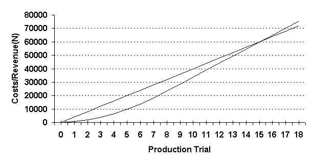
Plotting the data on the table into a graph in figure A. 1, it would be seen that the learning stage produced a non-linear curve between runs 0 to 7 and a perfectly linear relationship from run 8 onwards. These two characteristics made it possible for the total revenue curve to cut the total working capital usage line curve at the lowest possible point forming the break-even point at the N60,000 working capital requirement level. This is the least working capital requirement that can be considered adequate for the business given the company’s peculiar production and managerial characteristics. This can further be interpreted to mean that the company must have working capital enough to cover at least 15 production runs in order to make enough contribution margin to cover its 7 runs learning curve losses and continue with uninterrupted production.

Figure A.1 : Operational BEP Chart 1

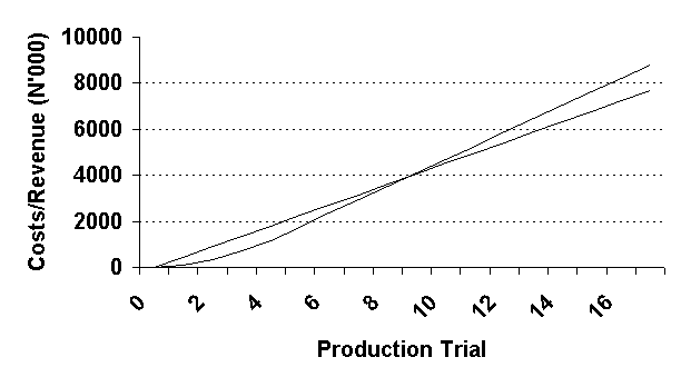
For further proof, the data for the beverage firm shall be similarly analysed and graphed. The firm operates a weekly production cycle which gives a weekly production cost is 452,000. Applying the above information we have the following data:

A = 452000

n = 5

m = 0.3

t ranged from 4 to 1 (i.e. 5 > t >0)

Table A. 2 (N’000) Learning losses and Production Recovery Table (BEVERAGES)

RUN COST LOSS RECOVERY SALES CUM CUM CUM

LOSS COST SALE

1. 452 361.6 90.4 117.52 361.6 452 117.52

2. 452 271.2 180.8 235.04 632.8 904 352.56

3. 452 180.8 271.2 352.56 813.6 1356 705.12

4. 452 90.4 361.6 470.08 904.0 1808 1,175.20

5. 452 0 452 587.60 904.0 2260 1,762.80

6. 452 0 452 587.60 904.0 2712 2,350.40

7. 452 0 452 587.60 904.0 3164 2,938.00

8. 452 0 452 587.60 904.0 3616 3,525.60

Source: Daily Production and Sales Records

Here the learning stage ended with the 4^th run and the POP was reached in the 5^th run.

Again we can see how the learning loss thinned off at the 4^th production run. Graphically, the same pattern is also discernible, thus producing its own operational break-even point at 4,000,000 working capital requirement level.

Figure A.2 : Operational BEP Chart 2

Formulating the Adequate Working Capital and Operation BEP Model

Using the available data, the operational Break Even point (in numbers of required production runs) leading to the required adequate working capital with A, t, n, and m as before can be formulated as follows:

Operational Break-Even point (BEP) = (fn (1+m)) / m

Minimum number of activity trial runs to reach Operational Break-Even Point

P = ((n - 1) (1 + m)) / 2m

Minimum working capital required to reach operational break even point

WC@ P = (A (n - 1) (1 + m)) / 2m

The learning Process Loss Factor “f” then comes to: f = ( n – 1)/2n

Total Expected Losses “L” due to “Learning Process” becomes;

An x (n-1) = An (n - 1) = A (n-1)

1 2n 2n 2

Proof 1: With A=4000, n =8, and m=0.3,

The BEP (in number of production runs) will be

P = ((8-1)(1.3)) / (2 x 0.3) = (7 x 1.3) / 0.6 = 9.1 / 0.6

= 15,167 runs (Approx. 16 runs)

The BEP in terms of working capital requirement will be:

WC @ P = (4000 (8-1) (3.1)) / (2 x 0.3) = 36,400 / 0.6

= N60.667 (Approx N61,000)

Compare these figures with those read from the graph in figure A. 1

Proof 2: With A = 452,000, n = 5, and m = 0.3

The BEP (in number of production runs) will be:

P = ((5-1)(1.3)) / (2 x 0.3) = (4 x 1.3) / 0.6 = 5.2 / 0.6

= 8.67 runs (Approx 9 runs)

The BEP in terms of working capital requirement will be;

WC @ P = (452000 (5 - 1) (1.3)) / (2 x 0.3) = 2.350.400 / 0.6

= N3,197,333 (N4million)

Compare the above figure with that read from the graph in figure A.2.

Significance of the operational Break Even Point:

The Operational Break Even Point is the point of activity where the internally generated revenue would have accumulated funds from Operations enough to recoup all losses attributable to the learning process and bring the organization’s working capital to an even keel, such that operations from this point onward adds more to profit and nothing to the reverse so long as the firm maintain the now attained level of efficiency and effectiveness in operation. This is the equilibrium position of the firm as regards its working capital position. Most importantly, the operational BEP is the point where it is now safe and convenient to repay back any borrowed fund used in augmenting the initial working capital base.

A good application of this concept will enable proprietors and managers to maintain a cautious and effective working capital base; deciding when to borrow and when to repay, when to expand activities and when to contract without affecting the firm’s operations. Also losses associated with work stoppages due to shortage of capital can conveniently be avoided if capital procurement and repayment is carefully planned and executed.

APPLICATION TO PROJECT EVALUATION

Applying this concept to the process of evaluating future project cost will enable a more reliable estimate of the total capital requirement of a project to be made in advance and adequate arrangement made to source the needed capital. The following mathematical model will assist in estimating the total capital requirement of a given project with a more cautious look and fairly high degree of accuracy.

Project Cost (P) = FC + WC @ BEP

Where

FC = Fixed or sunk cost of capital assets acquisition.

WC@BEP = Working Capital requirement at projects

Operational break - even point.

Revisiting the case of bakery, a proper capital requirement estimate for the company ought to be: P = (68,000 + 15,000) + 60,667 = N143,667, Compare this amount with the N115,000 the company has on commencement as revealed in the case study data. The short fall of N28,667 (i.e. N143,667 – N115,000) perhaps explains why it has to liquidate no sooner than it commenced operations.

Note: The working capital requirement of 60,667 was calculated using the

formula and figures in A.1

MEASUREMENT OF RELATIVE SOLVENCY.

Having calculated the required level of working capital for the business, it is now possible to measure the firm’s Relative Solvency Ratio (RSR) and the likely stage where solvency problem is expected to occur. This is calculated as follows: RSR = Available Capital / Required BEP Capital

Thus using the data for the bakery, its RSR will be measured as:

RSR = 32000 / 60667 = 0.5275

The probability or chance of liquidation is then measured as follows:

Chance of Insolvency (CI) = 1 - RSR

Thus, for the bakery, the chance of being insolvent = 1 – 0.5275 = 0.4725.

With CI determined, we may proceed to calculate the likely stage/point of production or trading when the insolvency is expected to occur.

This is simply measured by multiplying the RSR with BEP number of productions; i.e.

Likely Point of Insolvency = RSR * BEP (Number of Runs)

For the bakery, this will be: LPI = 0.5275 * 15.167 = 8

This could be interpreted to mean that the company may become insolvent just by the 8th production run; and this was exactly the case. Relative Solvency Ratio (RSR) is so called because the ratio measures the available working capital in terms of the required working capital.

CONCLUSION

To prove that a relationship exist between Relative Solvency Ratio (RSR) and organizational life span, we measured the correlation or relative association between the two data for 18 failed business organizations provided in appendix B. The calculation of relative association in Appendix B, using the Spearman’s formula reveal that there is a strong correlation between organisational relative solvency ratio (RSR) and its longevity as given by the correlation rate of 0.835.

A more stringent mathematical proof performed outside this article using a “t” distribution hypothesis test revealed that “The mean life of Organizations having RSR less than 1 is significantly different from those organizations having RSR greater than or equal to “1" this is to say that if those companies that failed were given the opportunity to know and improve on their relative solvency ratio (RSR) in terms of making more working capital available at their various points of need, the story could had been a lot different.

RECOMMENDATIONS

Though, this study was based on the data collected from business operations in Nigeria, we believe that this new concepts is of universal relevance. However, in order to provide a sound basis for its global acceptance/application, similar studies should be undertaken in other countries of the world. The researcher has a strong belief that the introduction and implementation of the findings of this research as additional tool of financial management with regards to working capital management would go a long way to improve the operational performance and relative longevity of most organizations.

BIBLIOGRAPHY

Altman E.I. (1983),,CORPORATE FINANCIAL DISTRESS - A Complete

Guide To predicting, Avoiding and Dealing with Bankruptcy, New - York, Willey

Argentini J (1969) CORPORATE COLLAPSE - The Causes and Symtoms,

New York, Fraeger.

Child J. (1969), BUSINESS ENTERPRISES IN MODERN INDUSTRIAL

SOCIETY, London, Collier - Macmillan

Doetsch D. A. & Hammer L. A. (2002), “OBSERVATIONS ON CROSS-

BORDER INSOLVENCIES AND THEIR RESOLUTION IN THE NAFTA

REGION”, United States and Mexico Law Journal, Vol. 6 @

www.mayerbrownrowe.com

Enyi E.P. (2002) WORKING CAPITAL MANAGEMENT - New Facts, Nkpor,

Panal Publishers.

Goldstick G. (1988) HOW TO GET IN THE BLACK AND STAY THREE. New

York, John Willey & Sons Inc.

Horngren C. T. (1982), COST ACCOUNTING - A Managerial Emphasis,

Englewood Cliffs, Prentice Mall Inc.

Nelson P.B. (1981) , CORPORATION IN CRISIS, Behavioural Observations

for bankruptcy Policy, New York, Fraeger,

Osisioma B.C. (1997), “SOURCES AND MANAGEMENT OF WORKING

CAPITAL”, Journal of Management Sciences, Vol. 2, Awka,

Nnamdi Azikiwe University

Pickles W & J.L. Lafferty (1974) ACCOUNTANCY, London, MacDonald &

Evans (E.L.B.S.)

Sellers E. A., MacParland & Hoffner F. J. (2002), “GOVERNANCE OF

FINANCIALLY DISTRESSED CORPORATIONS: New Challenges For

Refinancing in Global Capital Markets”, University of British Columbia

Bankruptcy Journal, Vancouver, Canada, February

Samuelson P.A. (1980), ECONOMICS, Tokyo, McGraw Hill Kogakusha Ltd.

VanHorne J.C. (1977) FINANCIAL MANAGEMENT AND POLICY

Englewood Cliffs, Prentice Hall Inc.

APPENDIX A

LIST OF SELECTED FAILED BUSINESS

ORG. CODE

TYPES OF BIZ

INCEPTION DATE

LIQUIDATION DATE

LIFE SPAN (MONTHS

RSR RATIO

CAUSE OF

DEATH & LOCATION

C03

D04

E05

F06

G07

109

J010

L11

L12

M13

N14

O15

P16

Q17

R18

S19

T20

V21

BANK

FINCOY

BANK

FINCOY

BANK

BEVMFR

BREW

MOTOR

BAKERY

BREW

BEVMFR

BREW

BKSHOP

1929

1931

1937

1933

1971

1993

1947

1986

1952

1989

1976

1978

1984

1980

1986

1980

1970

1930

1936

1994

1999

1994

1995

1953

1986

1960

1995

1997

1988

1984

1992

1990

1980

684

732

338

276

252

120

144

120

0.32

0.40

10.2

1.15

1.05

1.01

0.12

0.50

0.02

0.06

0.15

0.75

0.52

0.41

0.60

0.42

0.36

0.65

INSOL LAGOS

MIS-M LAGOS

INSOL NNEWI

INSOL LAGOS

INSOL ULI

INSOL ONITSHA

INSOL KANO

INSOL ENUGU

INSOL ABA

INSOL KANO

KEY: FINCOY = FINANCE COMPANY ; BEVMFR = BEVERAGE MANUFACTURER;

BKSHOP = BOOK SHOP; INSOL=INSOLVENCY; MIS-M = MISMANAGEMENT

(COMPANIES IDENTITIES CODED FOR CONFIDENTIALITY)

SOURCE: NATIONAL ARCHIVES IBADAN

RSR DERIVED FROM COMPANY’S ANNUAL REPORTS.

APPENDIX B

TEST OF CORRELATION BETWEEN COMPANY LIFE SPAN (IN MONTHS) AND RELATIVE SOLVENCY RATIO (RSR)

COY LIFE RSR

CODE SPAN (X) (Y) (XY) X² Y²

C03 12 0.32 3.84 144 0.1024

DO4 60 0.40 24.00 3600 0.1600

J10 24 0.12 2.88 576 0.0144

K11 72 0.50 36.00 5184 0.2500

L12 8 0.02 0.16 64 0.0004

M13 96 0.60 57.60 9216 0.3600

N14 72 0.15 10.80 5184 0.0225

015 252 0.75 189.00 63504 0.5625

P16 120 0.52 62.40 14400 0.2704

Q17 3 0.41 1.23 9 0.1681

R18 144 0.60 86.40 20736 0.3600

S19 72 0.42 30.24 5184 0.1784

T20 120 0.36 43.20 14400 0.1296

V22 120 0.65 78.00 14400 0.4225

E05 684 1.02 697.68 467856 1.0404

F06 732 1.15 841.80 535824 1.3225

G07 338 1.05 354.90 114244 1.1025

I09 276 1.01 278.76 76176 1.0201

TOTAL 3205 10.05 2798.98 1350701 7.4847

n = 18

r = 18 (2798.89) - 3205 (10.05)

Ö(18(1350701) - 3205²) (18(7.4847) – 10.05²)

= 18169.77 / 21759.56

= 0.835

This result shows a strong positive correlation between RSR and company life span.